
In this series you’ll find walk-throughs of several different projects which show how Python can be used effectively in mechanical engineering. The purpose of these walk-throughs is to give mechanical engineers a vision of how they can use Python in their own area of expertise and understand the scope of what is possible, whether for business or academia. As you walk through the showcase projects in this series you’ll also learn some of the different modes of writing and using python in an engineering environment – for example, we can use Jupyter lab for peer-reviewed calculations or we can package our code into a graphical desktop application or web application for use by other users. We’ll also introduce a number of key Python packages – additional add-ons to Python which extend the functionality of the language, such as matplotlib for plotting and visualizing data. If you’ve got suggestions for projects or topics please leave a comment!
Each walk-through begins with a description of the mechanical engineering scenario before the project walk-through. This is followed by an assessment of the benefits of using Python over traditional software, such as Excel, Matlab and MathCAD.
Although this series can be understood if you’ve never used Python before, the aim is not to teach basic python syntax nor to delve into all the details of scientific python packages.
Total beginners to Python should first start with a course such as Learn Python by Codecademy or Python Jumpstart by Building 10 apps by Michael Kennedy.
1. Installation
The walk-throughs in this series will be mostly based on the Anaconda distribution of Python. At the present time this is the most useful distribution for a number of reasons. Whereas software companies focused on Python would most likely program on the Linux operating system, the vast majority of engineering companies will be using Windows. However, Python installation and package management was previously not at all straightforward on Windows. In addition Python is open source and maintained by volunteers and therefore difficult to accept as a valid solution for some enterprise companies who require a guaranteed level of support.
Using Anaconda overcomes these issues – it has its own package manager built-in, and already has the most used scientific packages pre-installed, and also includes Jupyter Lab which can be used as a notebook or and integrated development environment, all from within a browser. In addition to this, you can download Anaconda for free on Windows, Linux and Mac, but you can also choose to pay a subscription for support.
To install, simply goto https://www.anaconda.com/, click download and follow the instructions for your platform. Remember to choose Python 3 (not legacy Python 2 which will soon be discontinued).
Introduction to Anaconda
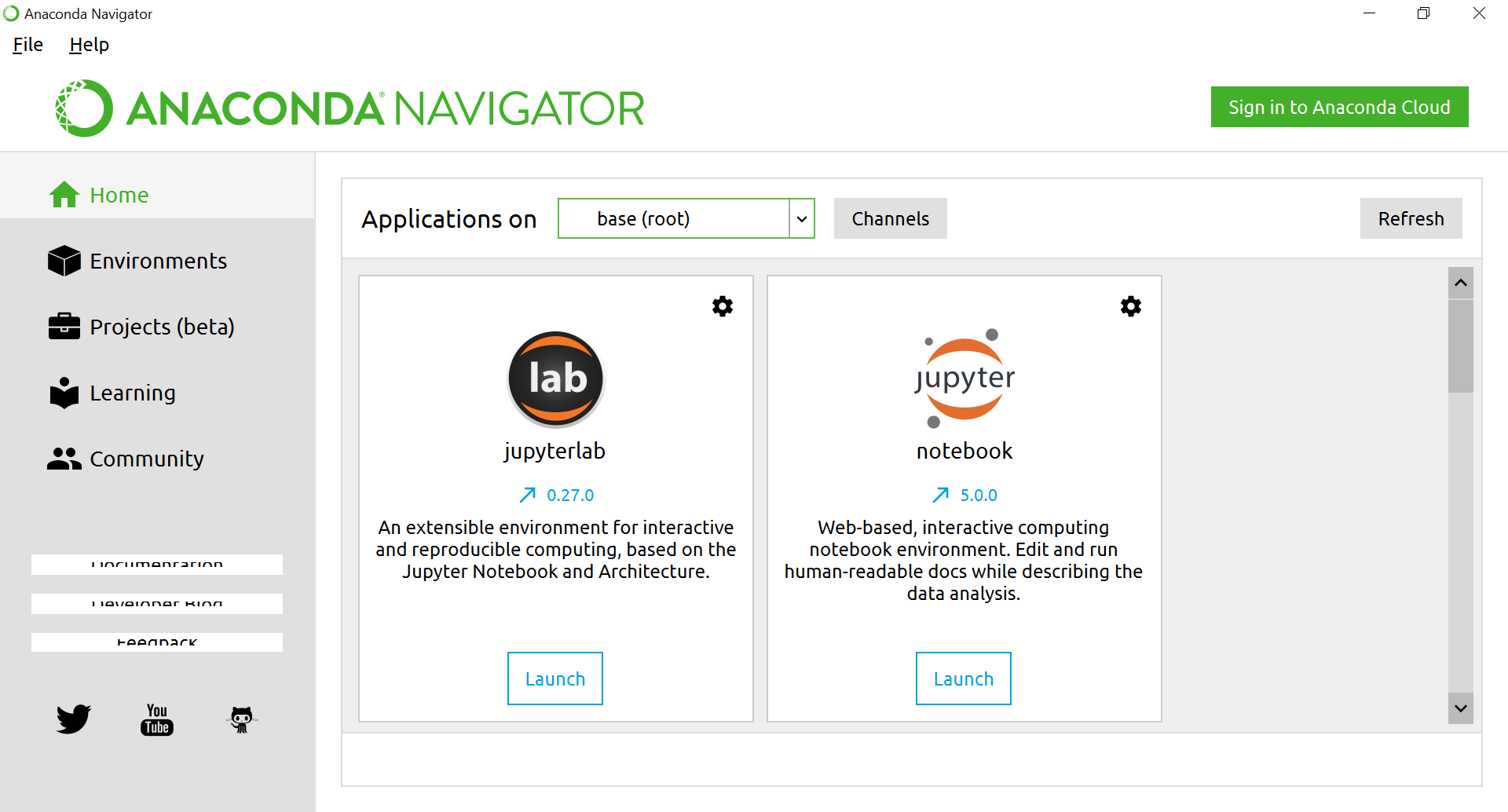
From the start menu open ‘Anaconda Navigator’
2. Home tab – Jupyter Lab
In the ‘Home’ tab you can launch the applications that come with Anaconda. We’ll mostly be using Juypter Lab. Click ‘launch’ and Jupyter Lab will be opened in your default web browser.
Jupyter Lab is a new integrated development environment, which we’re using in this series because it gives us the ability to use python in a number of different ways. In the left hand pane is a file manager along with some other tabs, giving you quick access to open files in Jupyter without leaving the browser.
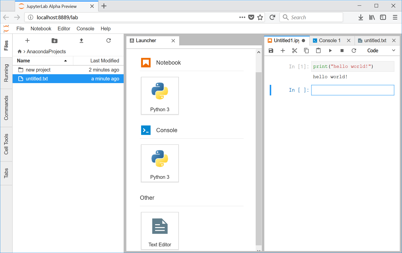
The Launcher pane gives us 3 different options:
a) Text Editor
The text editor is exactly what is says, and the core component of any development environment – its where you write your code. Of course you can write Python code in any text editor even notepad – but the advantage of a proper IDE like Jupyter is that your code will get syntax highlighting as you type, making it easier to read and debug. For example Python keywords are given one colour, text strings another and so on. We’ll use the text editor in later tutorials to create programs and web apps that might be deployed and used by others who don’t need to interact with the code itself but only the functionality.
b) Console
The console basically runs Python in interactive mode, with the <code>>>></code> prompt letting you know its waiting for some code. This mode immediate feedback for each statement, while holding previous statements in active memory – like running a script line by line. This is a great way to play around with Python to see how things work.
c) Notebook
The notebook is the main feature of Jupyter – its kind like an advanced version of a text editor and the console melded together, or as the official website explains: “The Jupyter Notebook ….allows you to create and share documents that contain live code, equations, visualizations and narrative text. Uses include: data cleaning and transformation, numerical simulation, statistical modeling, data visualization, machine learning, and much more”. The crucial feature for engineers is the ability to enter equations in mathematical notation as well as python code – giving you the power of python and the clarity of expressing things as you’d write them (and so has advantages over the traditional software which we’ll discover over the course of this series).
3. Environments
Anaconda environments work in the same way as Python virtualenvs – they acts as separate environments with their own set of packages relevant to your project. Whilst the standard Anaconda root environment comes with a number of pre-installed packages, you’ll doubtless need to install some additional ones.
Start by creating a new Anaconda environment by clicking ‘Create’ and entering a name. You can then install packages from the right hand side pane – choose ‘All’ from the dropdown list, and then search for the package you want. Check the box beside the package name and then click ‘Apply’ and your package will be downloaded and installed.
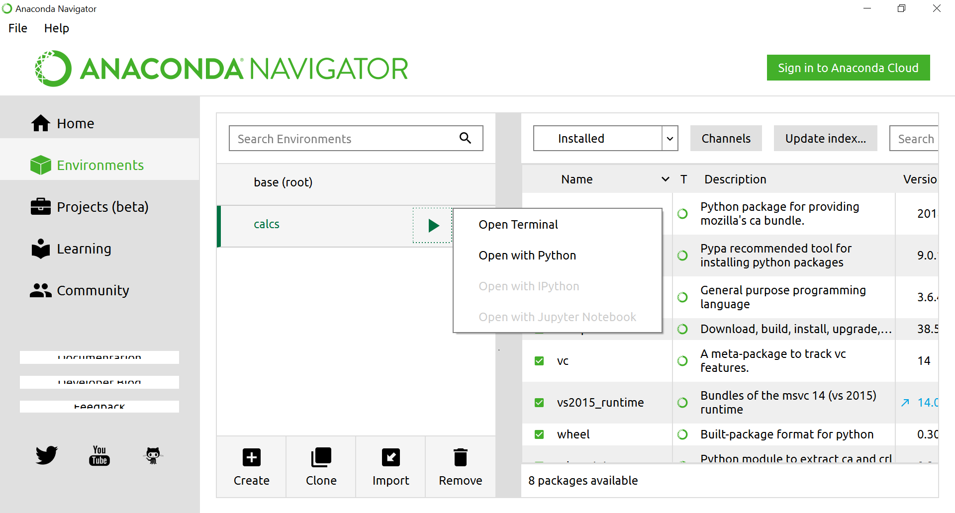
This list of packages in the Anaconda environment is curated, but you can also install anything from the python online repository (pypi) using the command line tool pip. If the package you want is not available within Anaconda, in the Environments tab, click the play symbol next to the environment you want to use (here named calcs), then chose ‘Open Terminal’. You’ll be presented with a terminal like this:
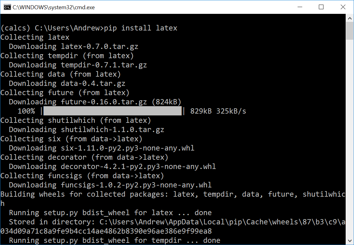
To install a package type the command:
pip install package_name
in this case we’re installing the package ‘latex’. You can click the ‘x’ or type exit and press enter to close the terminal.
In a later article we’ll look at a using git version control from within Jupyter and Spyder – the final piece of our toolkit for using Python on windows. However, coming up next we’ll tackle a real life mechanical engineering problem using the tools we’ve installed today.
Leave a Reply